VAE in 3D
In this tutorial, we are going to implement and visualize the training process of Variational Auto-Encoder with 🔗 Efemarai.
About Efemarai
Efemerari is a visualization and debugging tool for pytorch models. It works by scanning the model's forward and backward steps and visualizing the different modules, tensors and activations within a 3D environment right in your browser. Efemerari allows you to inspect all values of each tensor within the model computation.
What is VAE
Variational auto encoders are neural networks that learn to generate unseen data from a dataset by learning to map some known (latent) distribution to the unknown distribution of the datasets. The architecture of a VAE follows the general architecture of an auto-encoder, but also adds special module for sampling from the encoded distribution parameters. The optimization procedure of a VAE also adds special term to the loss to force the latent distribution to behave like a normal distribution.
The following is a diagram of a VAE:

Implementation
Let's get our hands dirty with some code.
1. The model
The implementation will be done in Pytorch.
We start by creating a torch module and add two
nn.Sequential
sub-modules for the encoder and the decoder.
class VAE(nn.Module):
    def __init__(self, input_shape, encoding_size):
        super(VAE, self).__init__()

        self.input_shape = input_shape
        flatten_size = np.prod(list(input_shape))
        encoding_size = encoding_size

        self.encoder = nn.Sequential(
            nn.Flatten(),
            nn.Linear(flatten_size, 16),
            nn.ReLU(),
            nn.Linear(16, 32),
            nn.ReLU(),
            nn.Linear(32, encoding_size * 2),
        )

        self.decoder = nn.Sequential(
            nn.Linear(encoding_size, 16),
            nn.ReLU(),
            nn.Linear(16, 32),
            nn.ReLU(),
            nn.Linear(32, flatten_size),
            nn.Sigmoid(),
        )

        self.loss = nn.BCELoss(reduction='mean')

    def forward(self, x):
      pass
Since the encoder is regressing to the parameters of some
normal distribution we are going to output
encoding_size * 2
number of parameters for $\sigma$ and $\mu$.
Let's now add functions for encoding and for decoding data.
class VAE(nn.Module):
    ...

    def decode(self, x):
        o = self.decoder(x)
        return o.reshape(-1, *self.input_shape)

    def encode(self, x):
        o = self.encoder(x)
        mu, log_sig = torch.chunk(o, 2, dim=1)
        return mu, log_sig
Notice how we chunk the output of the encoder into two vectors of parameters. These vectors correspond to the mean and variance of the distribution we are sampling from. Then we need a way to sample $z$.
2. Forward sample
class VAE(nn.Module):
    ...

    def sample(self, mu, log_sig):
        s = torch.normal(0, 1, mu.shape).to(DEVICE)
        return mu + s * torch.exp(log_sig / 2)
The thing we do in the sample method is called reparameterization and it allows us to make the sampling differentiable. Instead of directly generating a sample from the inferred parameters we sample a normally distributed vector from $N(0,1)$ and rescale and shift it accordingly.
And finally, lets implement the forward method.
class VAE(nn.Module):
    ...

    def forward(self, x):
        mu, log_sig = self.encode(x)
        s = self.sample(mu, log_sig)
        out = self.decode(s)
        return out
3. Dataset
Now we need a dataset. Lets go with the classic - MNIST. Luckily torchvision makes this super easy.
dataset = torchvision.datasets.MNIST(
    root='./data',
    transform=transforms.Compose([
        transforms.ToTensor(),
        transforms.Lambda(lambda x: x[0])
    ]),
    download=True
)

mk_data_loader = lambda bs: torch.utils.data.DataLoader(
    dataset=dataset,
    batch_size=bs,
    shuffle=True
)
4. Optimization loop
After that we initialize our model and we are ready to toss it in whatever training loop framework we like. In my case that is this simple optimization function.
def optimize(model, data, epochs, lr=0.01, on_it=lambda _: None):
    optimizer = torch.optim.Adam(model.parameters(), lr=lr)

    tr = trange(epochs)
    for epoch in tr:
        for i, (X, y) in tqdm(
            enumerate(data),
            total=len(data),
            desc='Epoch [%i/%i]' % (epoch + 1, epochs)
        ):
            X = X.to(DEVICE)

            optimizer.zero_grad()
            loss = model.criterion(X)
            loss.backward()
            optimizer.step()

            tr.set_description('Loss %.6f' % l)
We are ready to optimize!
loader = mk_data_loader(bs=64)
vae = VAE(X[0].shape, emb_size).to(DEVICE)

optimize(
    model=vae,
    data=loader,
    epochs=5,
    lr=0.01
)
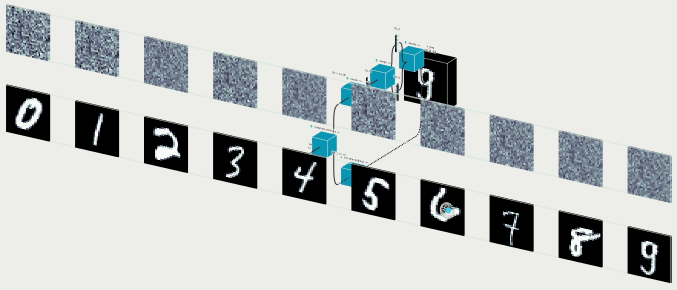
Visualizing the training with Efemarai
Lets install the python package of efemarai:
export EFEMARAI_LICENSE_TOKEN=<your-license-token>

pip install efemarai \
  --extra-index-url https://${EFEMARAI_LICENSE_TOKEN}@pypi.efemarai.com
After that we are ready to launch the efemarai demon.
Running the daemon locally ensures that none of your data, code or models leave your computer.
efemarai

> Daemon started successfully (use Ctr+C to exit).
After that to visualize the whole computation graph during training with
Efemarai, we just have to execute the model backwards step in
ef.scan like so:
import efemarai as ef

def optimize(...):
    ...

    with ef.scan(wait=i==0):
        loss = model.criterion(X)
        loss.backward()

    ...
In my case I add wait=i==0,
to make the execution of the code break on the first iteration.
This ensures that we can expand the graph in the
web interface before the training begins.
Now is the time for us to navigate to the web interface of Efemarai at app.efemarai.com/run. You should be greeted with the following screen:
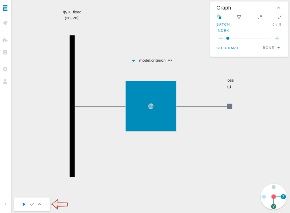
You can drag with left mouse click while holding Shift to rotate and drag with right mouse click with Shift to pan. Click on the blue boxes (operations) on the graph to expand them.
Step by step in the web interface
Conclusion
In this post we saw what VAE is, how to implement one and how to visualize it. I encourage you to try the experiment yourself and play around with the visualization interface of Efemarai. You can also try it with models you have already implemented. The code necessary for the visualization to work is literally a few lines.