Emergent structures in noisy channel message-passing
In this blog post we will explain a mechanism for generating neural network glyphs, like the glyphs we use in human languages. Glyphs are purposeful marks, images with 2D structure used to communicate information. We will use neural networks to generate those structured images. The basic idea is rather simple and the principles at play can be explained easily.
Source: ResearchGate
We want to generate images, containing visuals information, much like the images from the MNIST dataset. So what constitutes something that can be recognized in an image? Well, images are grids of pixels with close values being highly correlated. Also, images are robust to perturbations, visual noise, translations, rotations, and more. Meaning the information contents of an image is mostly preserved under those transformations. So what can we do if we want to generate images with these properties without any sort of dataset? We can optimize for robustness. But what do I mean by that?
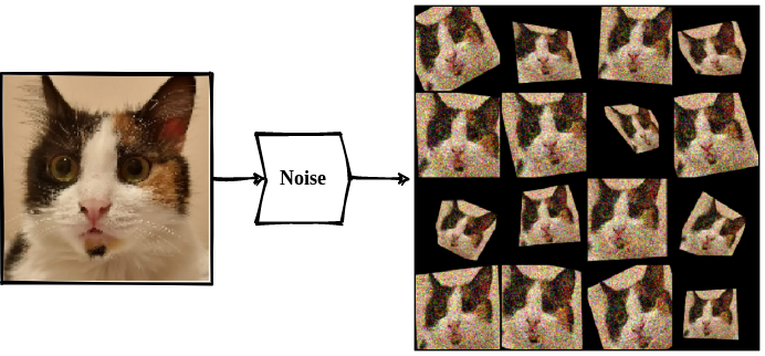
This is the training procedure we will follow the model of this diagram:

- Generate a random vector, a message.
- Expand the message with a generator (possibly
conv-transposemulti-layer network) generating an image from the initial message. - Induce differentiable noise into the image. Examples of such noise transformations include:
- Translation
- Rotation
- Crop
- Arbitrary UV-remap (being differentiable with the use of
spatial transformer) - Multiplying or adding normal noise
- Compress the disrupted image with a decoder (possibly conv multi-layer network) resulting in new vector a predicted message.
- Minimize the distance between the input and the predicted message.
In this way, we are optimizing the generator to generate images that can be “understood” (decoded) even if perturbed. Depending on the noise under which we optimize the generator learns to induce robustness into the images. It adds patterns with high dimensionality which are used to communicate the information contained in the input message. As a neural network architecture, this looks like an Inverted Auto-Encoder and it is trained exactly like a regular AE.

The image of the cat in the diagram is just an example. The network would not actually learn to generate cats.
The networks are basically communicating normally distributed points from ${\Bbb R}^{N}$, where $N$ is the size of the message.
The model is the same as an Auto-Encoder, we just swaps the positions of the compressor, commonly known as Encoder, but here it is named Decoder since it decodes the initial message, and the generator,
commonly known as Decoder, but here it is named Generator since it generates the image.
The generator has to learn to generate images that still contain the original information of the message after they are augmented.
Generating structure from nothing
To define and train the model we will be using PyTorch, modern and powerful library for all things Deep Learning. For the differentiable noise function we will use Kornia, because it has useful computer vision functions commonly used in data augmentation.
The full code of this project can be found in this repo: inverted-auto-encoder.
The architecture can be summarized with the following - a few activated and batch normalized ConvTranspose2d layer for the Generator
and activated and batch normalized Conv2d layers for the Message Reconstruction network.
Between them we place sequence of kornia random augmentation differentiable modules like so:
img = load_img(url, size=512)          # Load
img = img.unsqueeze(0).float() / 255   # Normalize
imgs = T.cat(16 * [img])               # Add multiple in batch
normal_noise = T.randn_like(imgs) / 4  # Generate random noise

noise = nn.Sequential(
    kornia.augmentation.RandomAffine(
        degrees=30,
        translate=[0.1, 0.1],
        scale=[0.9, 1.1],
        shear=[-10, 10],
    ),
    kornia.augmentation.RandomPerspective(0.6, p=0.5),
)

augmented_imgs = noise(imgs + normal_noise)

imshow(augmented_imgs)
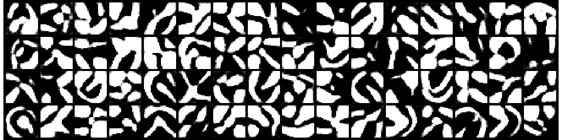
This definition of the augmentation function can yields results similar to these:
We have random affine and perspective transformations. The normal noise added before the augmentation is also an important component as it leads to the generator learning to generate smoother images.
For the data we will be using the following message generator:
msg_size = 64

def sample(bs):
    return T.randn(bs, msg_size).to(DEVICE)

def get_data_gen(bs):
    while True:
        X = sample(bs)
        yield X, X
We generate randomly distributed vector with msg_size dimensions and we yields tuples of this vector replicated as we will train
our model just like an Auto-Encoder.
We are ready to toss the model and the data generator in our favorite PyTorch training loop framework.
In my case that is a simple home brewed library that is part of the code in the repository of the project.
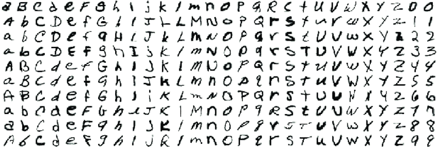
Lets fit and plot the generated images as we train!
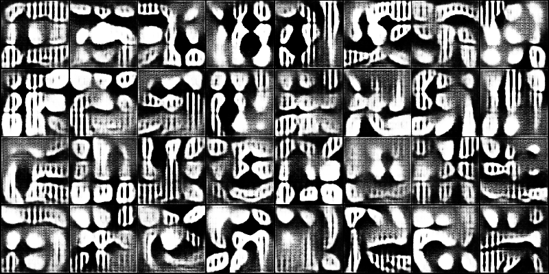
 The final result of the generated images from initial message sample.
If we try to cram the same amount of information - normally distributed vectors with size 64 into a 100x100 images we get the following result.
Voila, we got something. Let’s now try to progressively increase the message size and view how that changes the generated images. The idea is that this might force the generator to generate objects with higher level of detail, since it has to cram more information into the same image size.
The generated images are with size of the message 32, 128, 512 and 1024 respectively:
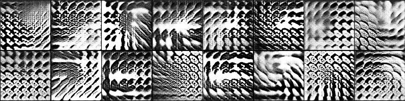
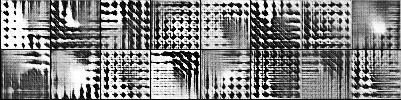
We get pretty images with some sort of structure in them. Lets continue with the experiments.
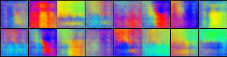
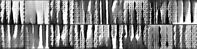
Adding color
Now lets add three channels to the generated image and see what kind of colorful patterns the
network will generate. The following images are generated from networks trained with messages
with dimensions 32, 128, 512, 1024 and 2048 respectively.
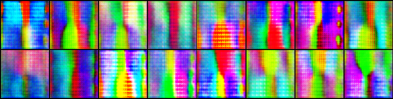
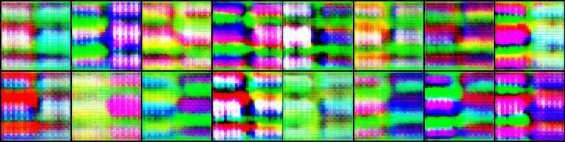
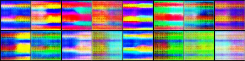
Pretty cool, but I don’t think I see a pattern of increasing complexity as I was expecting.
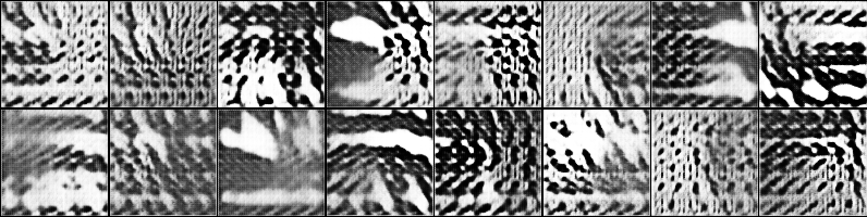
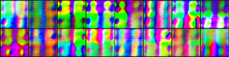
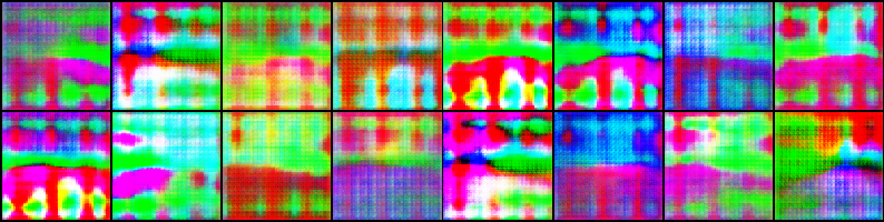
Interpolating in latent space
For our next visualization, lets sample multiple points (symbol representations) and
interpolate between them, interpolating also between the generated images.
We see structural changes in the shapes generated by the network, meaning the information in the message vector is being interpreted as higher level features in the image.
Usefulness of the model
An interesting question I think is worthy of an experiment is: Can these networks give useful representations to natural images? To answer this question we must first answer what constitutes a good representation. We will try to evaluate the usefulness of the network and the representations it extracts in the following ways:
-
Invert the
generatorand themessage decoder, as they would be in an ordinaryAEand try to reconstruct images from the MNIST dataset. Bare in mind the network has never seen natural images. -
Use the representations from the
message decoderto squeeze the images from MNIST and train a classifier over these representations. We can compare against randomly initialized generator and see which trains faster and to what accuracy expecting out image generating network to do better. -
We can also try to find representations generating valid MNIST images by doing gradient descent over the input representation of the generator, with a loss differentiating between the output of the generator and a particular MNIST image. Basically searching for messages which generate the digits of MNIST.
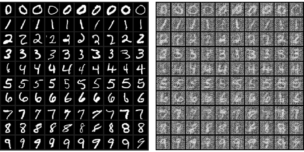
Reconstructing MNIST
Inverting the inverted auto encoder and reconstructing MNIST we get the following. Focus on the middle and the right image.

It is evident that the network can not reconstruct the images in understandable manner, but from the example above we can see that all images from the same class are “reconstructed” with similar shapes, which is interesting.
Training a classifier over the zero supervised representations
For this experiment we trained four instances of the model with different configurations with single trainable linear classifier on top of the decoder.
We have pre-trained decoder (with the noise scheme described above) vs a randomly initialized one. We also have frozen decoder vs decoder with non-frozen weights. Running SGD multiple times we get the following:
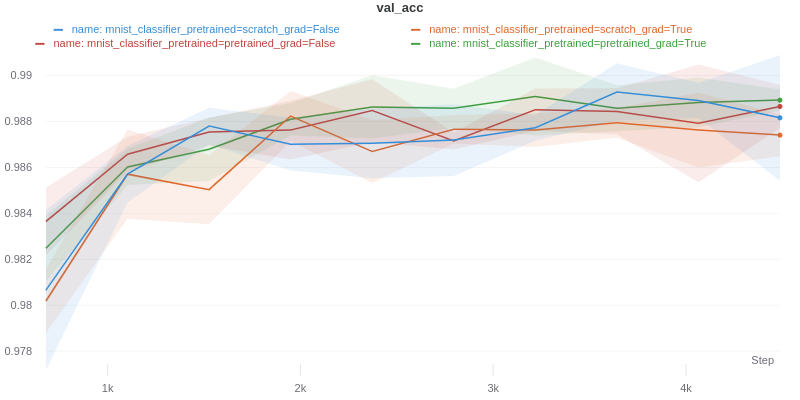
Bummer. No difference in the slope of the different instances of the model is noticed, meaning we cannot verify the representations from the zero-shot pre-trained model are “better” for the described definition of better.
Generating natural images optimizing the input
For this final experiment lets freeze the network weights on both trained and randomly initialized image generator and optimize a set of input vectors to generate a single batch of predefined MNIST images. The hope is that the optimization with the trained generator will be able to find vectors generating the set of MNIST images, since the trained generator can generate some sort of structure.
Running this experiment we get the following results:
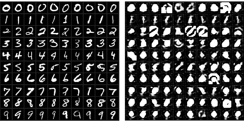
Images generated by the pre-trined generator have structure in them, but the digits are not recognizable, they are mostly blobs without detail.
With this observation we can sadly conclude that the network has NOT learned anything “useful” for actual natural images, for the described definition of useful. But we still got a fun AI ART project 😊.

In the next post we will experiment with AE as augmentation function. For now we could not show that
this zero-shot training setup is nothing more than interesting way of generating abstract neural network art,
which depending on your interests could also be something you would like to try.
For details on the implementation of the models and the experiments check out the repo of the project. This project was highly inspired by GlyphNet by Noah Trenaman. You should definitely check out the repo.