Generating random art with neural networks
Recently, I discovered blog.otoro.net - David Ha’s blog and I was delighted to see all kinds of creative applications of deep learning. In this post, I will attempt to replicate and build on top of his work on CPPNs. As this post is heavily inspired by the articles of the blog mentioned above I strongly recommend that you read them as well.
What is CPPN
First things first, what is a Compositional Pattern Producing Network.
The Wikipedia definition is as follows:
Artificial neural networks that have an architecture whose evolution is guided by genetic algorithms.
Well, in the current post I would not be doing anything related to genetic algorithms. The architecture of the networks would not be evolving and neither is the topology of the computation be anything more than a vanilla feed-forward network as the FFN would be enough to produce interestingly looking results. What the network is going to do is take a discrete 2D vector field (mesh grid) and map it to the 3D space of colors.
\[f: {\Bbb R}^2 \to {\Bbb R}^3\]Since the input mesh grid will be somewhat smooth as viewed in a 2D matrix
and because the neural network is continuous function,
we would expect the results to resemble random, but smooth transitions between colors.
In a sense, the neural network would act as a fragment shader just like the one you
have in Shadertoy. Taking in the uv coordinates of the pixels
and mapping them to colors.
Here $a$ is some activation function (like $tanh$ or $\sigma$) and $\sigma$ is the sigmoid function. We naturally activate the last layer with $\sigma$ so that we map the output is in the range $(0, 1)$.
Since the network would not be trained the output would depend on the random initialization of all the parameters of the network hence - generating random art. We would extend this by adding a random (latent) vector as an input which would vary the generated image. The vector would be fixed for the pixels of a single image but varied in time leading to smooth animations.
Implementation
Let us use pytorch to construct the mapping. We will start by defining a function that
will create a Dense layer - affine transformation followed by activation.
import torch
import torch.nn as nn

def dense(i, o, a=nn.Sigmoid):
    l = nn.Linear(i, o)
    l.weight.data = torch.normal(0, 1, (o, i))
    l.bias.data = torch.normal(0, 1, (o,))

    return [l, a()]
Notice the normal initialization. It is important for the region of space that we sample from
namely - ${\Bbb R}^2$ around (0, 1).
You can experiment sampling from different distributions, but some of them might not make sense
for the range in question.
After that, we can create a feed-forward network class that is defined by its
width and depth.
class FFN(nn.Module):
    def __init__(self, width, depth):
        super(FFN, self).__init__()
        self.net = nn.Sequential(*[
            *dense(2, width, nn.Tanh),
            *[l for _ in range(depth - 2)
                for l in dense(width, width, nn.Tanh)],
            *dense(width, 3, nn.Sigmoid),
        ])

    def forward(self, x):
      return self.net(x)
That’s all that we need in terms of a network. Now let’s create the input.
steps = 512
l, r = 0, 1
x = torch.arange(l, r, (r - l) / steps)
y = torch.arange(l, r, (r - l) / steps)
xx, yy = torch.meshgrid(x, y)
inp = torch.stack((xx, yy), dim=-1)
meshgrid broadcasts the vectors to a matrix. After that we stack them
to obtain 2D grid of 512x512 uv coordinates between 0 and 1.
Let’s continue by initializing the network. We pass the colors one by one
by reshaping them into a (steps*steps)x2 matrix - each color is a separate input.
After that, we reshape the output back to 255x255x3 to get the final image.
model = FFN(width=25, depth=9)
output = model(inp.reshape(-1, 2)).detach().numpy()
output = output.reshape(steps, steps, 3)
output.shape
>> ((512, 512, 2), (512, 512, 3))
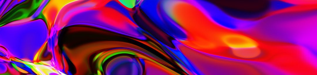
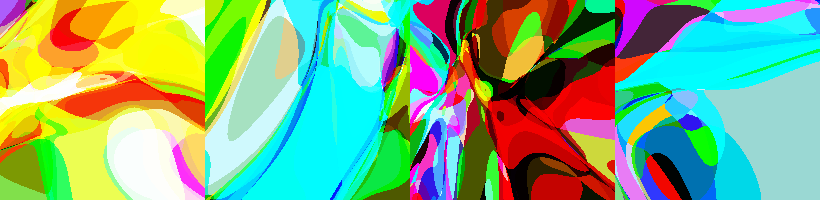
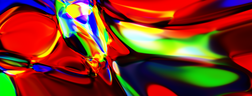
And we are done! Now let us see what the random initialization gives us as output.
import matplotlib.pyplot as plt

plt.imshow(output)
Looks pretty good to me!
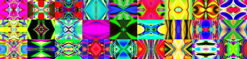
Playing with the parameters
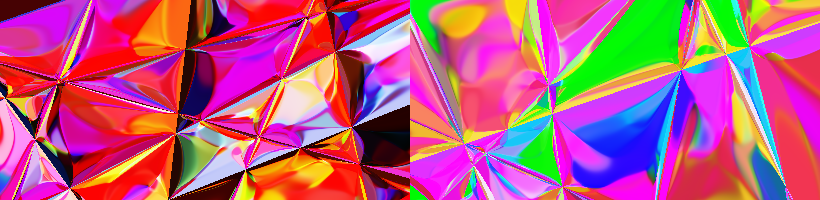
These were obtained by varying:
- The width and depth parameters
- The activations of the network at different levels
- $tanh$ - silky output
- $tan$ - sharp transitions
- $sin$ - frequent but smooth color change
- $sign$ - single color regions
- The size of the output (1 - monochromatic, 3 - colorful)
Variations on the theme
That’s all cool and all, but how can we spice things up.
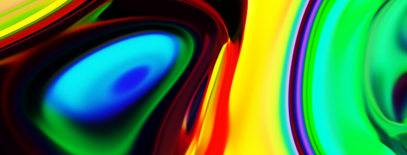
Animation
We can animate these mappings by adding another input vector $z$ of arbitrary size ($N$) that is constant for the whole image. Interpolating between two point in ${\Bbb R}^N$ and producing different images from that will yield smooth animations.
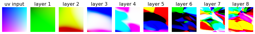
\[f(u, v, z_t) = \sigma(...W_2 a(W_1 [\vec{uv}, \vec{z_t}] + b_1) + b_2...)\]Here $[.,.]$ denotes vector concatenation. You can easily extend the code above to achieve this result or you can also look at the reference notebooks. As for the results, it really depends on the architecture of the network and the distributions that is used to seed the weights and biases. In general, you can expect to see something like this.
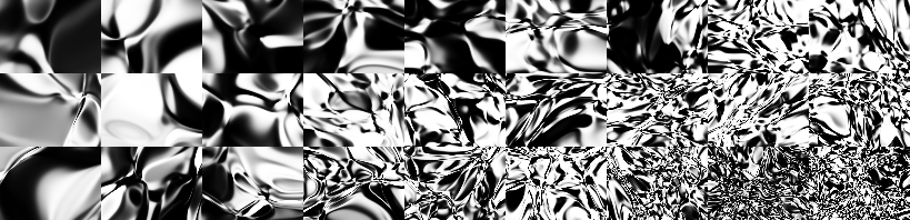
If we vary the depth and width parameters along the x and y axis we get something like this.
Super-sampling
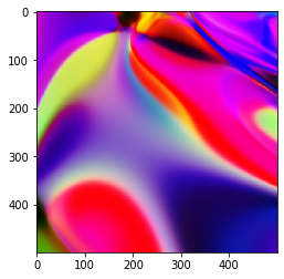
Each image is represented as matrix of colors. This means that we can view our image as sampled from a ${\Bbb R}^2 \to {\Bbb R}^3$ function. Since all of the operations in our CPPN are differentiable we can train it to approximate any image with standard gradient descend. We can imagine our network as training to map the location of each pixel to the three channels of the image. This can be though of as simple supervised curve fitting for a 2D function.
At the end of the training we can sample our network with higher (infinite) density, limited only by the precision of the floating point calculations. But we cannot expect much from this model. Since each pixel is generated considering only its location, plus the fact that we would train with a single image, the best that the network can do is to interpolate smoothly between the pixels. Unlike a CNN for super-resolution having some sort of semantic context (in the deeper layers) and inferring structure from this context our network could predict unexpected values between the learned pixels, only as a result of the randomness of the initialization and the stochasticity of the optimization procedure.
Why are we doing it then? Because its fun and we can visualize the process of training, which is pretty nice looking if you ask me.
This we will do with tensorflow, because why not.
def mk_model(depth, breadth):
    def block(u, a):
        return K.Sequential([
            K.layers.Dense(
                u,
                activation=a,
                kernel_initializer=tf.random_normal_initializer(0, 1),
                bias_initializer=tf.random_normal_initializer(0, 1)
            ),
            K.layers.BatchNormalization(),
        ])

    model = K.Sequential([
        K.layers.Input((2,)),
        *[block(breadth, a='tanh') for _ in range(depth)],
        K.layers.Dense(3, activation='sigmoid'),
    ])

    model.compile(
        optimizer=tf.optimizers.Adam(learning_rate=0.001),
        loss=tf.losses.BinaryCrossentropy(label_smoothing=0),
    )

    return model
The model itself is really simple. Just rewritten version of what we had for pytorch.
And for the training a single call to fit would be enough.
model.fit(
    mk_dataset(im, bs=1),
    steps_per_epoch=64,
    epochs=5,
    callbacks=[on_epoch_begin(lambda: show_sample(model, 32, 32, s=2))]
)
You can refer to the notebooks at the end for the full implementation and more examples.
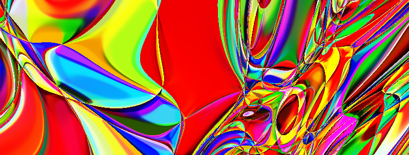
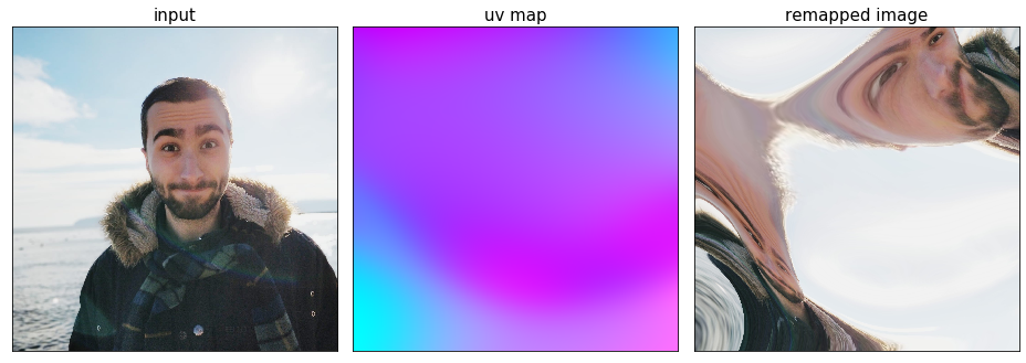
UV Remap
Now, instead of predicting the color of the output we can predict where to remap each pixel. Instead of outputting color, for each location we are going to output a new 2D location between 0 and 1, specifying where to sample the original image from at this location in the matrix.
This in graphics programming is called a uv texture map - image each pixel of which is specifying position in a texture corresponding to color for that particular location.
In short - we input the location of a pixel and the network tells us the location from which we have to sample some texture in order to obtain the color for that particular location.
This can be achieved by changing the size of the output of our current model to 2. Then we can do something like this:
uv = model(width=50, depth=7).predict(im_size=(W, H))
xx = uv[:, :, 0]
yy = uv[:, :, 1]

# Normalize the output
norm_xx = (xx - np.min(xx)) / (np.max(xx) - np.min(xx))
norm_yy = (yy - np.min(yy)) / (np.max(yy) - np.min(yy))

texture = cv2.imread('texture.jpg')
W, H, _ = texture.shape
remapped_image = cv2.remap(
  texture,
  norm_xx * W, norm_yy * H,
  cv2.INTER_AREA  # How to interpolate between pixels
)
For more details refer to the notebooks at the end.
And as before we can add random input vector fixed for all the pixels and vary it in time.
Adding symmetry to the input
We can make our outputs symmetrical by constructing the input as meshgrid from -1 to 1 and then taking the
absolute value of the coordinates.
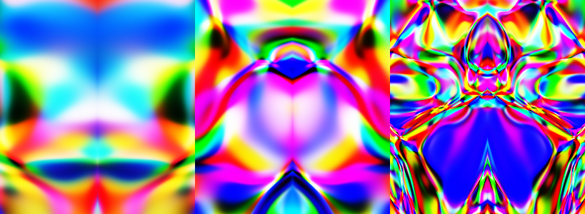
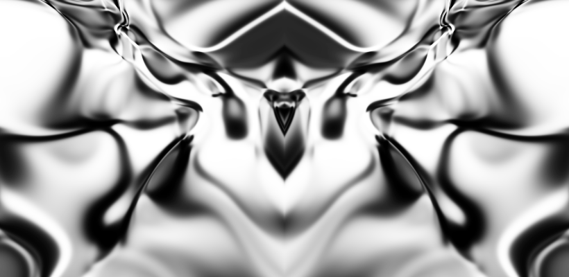
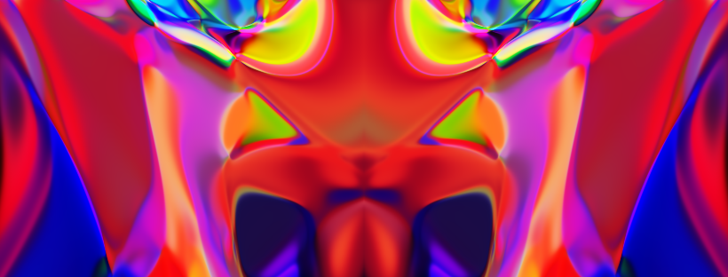
This is the same as taking the output image and mirroring it around one or two of its axis. Really simple, but the generated images look mesmerizing. Also, the outputs with $x$ symmetry are sometimes reminiscent of Rorschach images.
Conclusion
It is really interesting to see so much variety in the output of the CPPNs. There is a lot more to be explored here:
- Applying this technique in a 1D setting cold probably yield structure in audio - generating music
- The technique can be used to visualize latent vectors without 2D structure in matrix form (with 2D structure)
- Ha also explores different optimizing procedures leading to varying results
Although not very applicative these models are really fun to play with, so I encourage you to try running the notebooks yourself with different initial conditions or even better - implementing everything from scratch.